A ParaView tutorial for parallel visualisation

In ParaView, the prefix "Para" stands for "parallel" : How can we activate parallelism in ParaView ?

How to use this tutorial

  • This tutorial works only with the release 5.4.1 of ParaView
  • If you have data to be visualized by ParaView, you can use your data.
  • If you don’t have data yet, you can use some little scripts [23] written in python :
    • first, copy the scripts to your personal disk space :
    • When ParaView is started (see lower), you can read one script with the menu item : Tools/Python shell/Run script

Starting a graphics session

ParaView must be used from a graphics session. Because we want to visualize very big datasets, we probably need more memory than the default. We must also specify that we want more than 1 core.
The complete story is here. You can use the following command to start a graphics session :

  • using 25% of the graphics node’s cores
  • using 25% of the graphics node’s memory
  • with a comfortable display (if the width and the height of your workstation is sufficient)

Starting a visualization server

The ParaView gui [24] cannot use several cores. Only the readers and the visualization engines can use several cores. So we must start a server process, using mpi to make it to work in parallel. As we have 5 cores in this session, let’s dedicate 4 of them to server, keeping 1 core for the gui.
Open a terminal and type the following :

Starting the ParaView gui

Start ParaView version 5.4.1, using the main graphics menu : put the mouse over the root window, click with the right button, and choose the item Visualization_Applications/Paraview_5.4.1

Configuring the connection

The procedure described here should be done only the first time : the configured connection(s) will be kept from session to session.

  • When Paraview is started, click on the menu item : File/connect
  • A window entitled Choose Server Configuration opens, click the button Add Server
  • A window entitled Edit Server Configuration opens with several fields, all fields being already filled. Modify the value of the field Name, writing the name you choose for the connection : say my_pvserver, then click the button Configure
  • A window entitled Edit Server Launch Configuration opens, just click the button Save

Connecting to the pvserver

If not already done, start Paraview and click the menu item : File/connect, then select the my_pvserver line and click the Connect button. You are now connected to the pvserver, as PNG
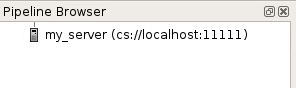
indicated in the Pipeline browser window (see figure). Besides, if you look at the window from which you launched pwserver, you should see this message :

Loading and displaying data

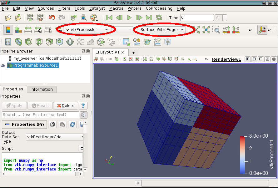
Figure obtained with 4 processors, using the python script rectilinear.py

You can now load your datafiles, your state files, your python scripts, exactly as usual.
Warning : to read a python script, you must use the menu item : Tools/Python shell/Run script.
Data will be read by pvserver, and rended and displayed by ParaView. You should have a new property available with your data : vtkProcessId

You can easily display the domain decomposition made pvserver for reading your data (see the figure).

If you execute a filter, it will be executed by pvserver, thus using several cores, which can lead to faster execution if you have a huge quantity of data to treat

Voir aussi

Bibliothèques scientifiques

FFTw HDF5

Logiciels scientifiques

Gaussian MEEP

Se connecter à EOS

Se connecter à Eos À partir de la plupart des réseaux académiques toulousains, on peut se connecter sur EOS par ssh :

L’espace-disque

L’espace disque d’EOS L’ espace disque d’EOS est constitué de trois espaces différents, chacun a une utilisation spécifique.

Lancer un calcul sur EOS

Lancer un calcul sur EOSLe mode interactif Pour la phase de mise au point

Documentations obsolètes concernant eos

L’uvprod (obsolète)

Améliorer les performances

Améliorer les performances de vos codes Vous trouverez dans cette rubrique différents moyens de déboguer votre application, d’améliorer les performances et d’optimiser un calcul sur le système de calcul EOS.

Comment fonctionne le système de Modules

Les commandes module permettent de personnaliser son environnement en termes de compilateurs, librairies, application (calcul, visu, etc...) de manière extrêmement simple.

ParaView

Lancement de ParaView Obligatoirement à partir d’un nœud graphique. Attention Si l’environnement openFoam est lancé, la commande ParaView n’est pas disponible : utilisez plutô

EOS schématisé : un peu de vocabulaire

Les termes techniques permettant de caractériser les différentes parties du supercalculateur

Gaussview

Utilisation de Gaussview Positionner l’environnement gaussian comme indiqué dans l’article sur Gaussian, puis :

XCrySDen

Lancer XCryDen à partir du menu graphique ! Ou... Lancer XCrysDen sur la frontale :

Jmol

Jmol est un outil de visualisation de molécules Lancer Jmol à partir du menu graphique Ou... lancer Jmol en ligne de commande :

gabedit

Pour l’utiliser : [@eoslogin1] gabedit

chdb, an MPI application for embarrasingly parallel problems

Embarrassingly parallel problems An embarrassingly parallel problem is a problem for which little or no effort is required to separate the problem into a number of parallel tasks [

compiler ses codes sur EOS

Le système de calcul EOS utilise le système d’exploitation linux. Ainsi deux environnements de compilation sont disponibles :

Une simulation en vidéo

Cette page présente une démonstration synthétique de l’usage du supercalculateur EOS.

Salome

SALOME propose des outils de pré/post-traitement et de couplage de codes de calcul pour la simulation numérique, ilintègre un module de visualisation (qui repose sur paraview).

VisIt

Lancement de VisIt Obligatoirement à partir d’un nœud graphique. VisIt est accessible à partir du menu graphique visit est également utilisable en ligne de commande :